Some examples of model hyperparameters include:

1. The penalty in Logistic Regression Classifier i.e. L1 or L2 regularization
2. The learning rate for training a neural network.
3. The C and sigma hyperparameters for support vector machines.
4. The k in k-nearest neighbors.

The aim of this article is to explore various strategies to tune hyperparameter for Machine learning model.

Models can have many hyperparameters and finding the best combination of parameters can be treated as a search problem. Two best strategies for Hyperparameter tuning are:

• GridSearchCV
• RandomizedSearchCV

GridSearchCV
In GridSearchCV approach, machine learning model is evaluated for a range of hyperparameter values. This approach is called GridSearchCV, because it searches for best set of hyperparameters from a grid of hyperparameters values.

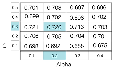
For example, if we want to set two hyperparameters C and Alpha of Logistic Regression Classifier model, with different set of values. The gridsearch technique will construct many versions of the model with all possible combinations of hyerparameters, and will return the best one.

As in the image, for C = [0.1, 0.2, 0.3, 0.4, 0.5] and Alpha = [0.1, 0.2, 0.3, 0.4].
For a combination C=0.3 and Alpha=0.2, performance score comes out to be 0.726(Highest), therefore it is selected.

Following code illustrates how to use GridSearchCV

Output:

Tuned Logistic Regression Parameters: {‘C’: 3.7275937203149381}
Best score is 0.7708333333333334

Drawback : GridSearchCV will go through all the intermediate combinations of hyperparameters which makes grid search computationally very expensive.
 
RandomizedSearchCV
RandomizedSearchCV solves the drawbacks of GridSearchCV, as it goes through only a fixed number of hyperparameter settings. It moves within the grid in random fashion to find the best set hyperparameters. This approach reduces unnecessary computation.

Following code illustrates how to use RandomizedSearchCV

Output:

Tuned Decision Tree Parameters: {‘min_samples_leaf’: 5, ‘max_depth’: 3, ‘max_features’: 5, ‘criterion’: ‘gini’}
Best score is 0.7265625

Decision Tree Classifier for building a classification model using Python and Scikit

Decision Tree Classifier is a classification model that can be used for simple classification tasks where the data space is not huge and can be easily visualized. Despite being simple, it is showing very good results for simple tasks and outperforms other, more complicated models.

Article Overview:

• Decision Tree Classifier Dataset
• Decision Tree Classifier in Python with Scikit-Learn
• Decision Tree Classifier – preprocessing
• Training the Decision Tree Classifier model
• Using our Decision Tree model for predictions
• Decision Tree Visualisation

Decision Tree Classifier Dataset

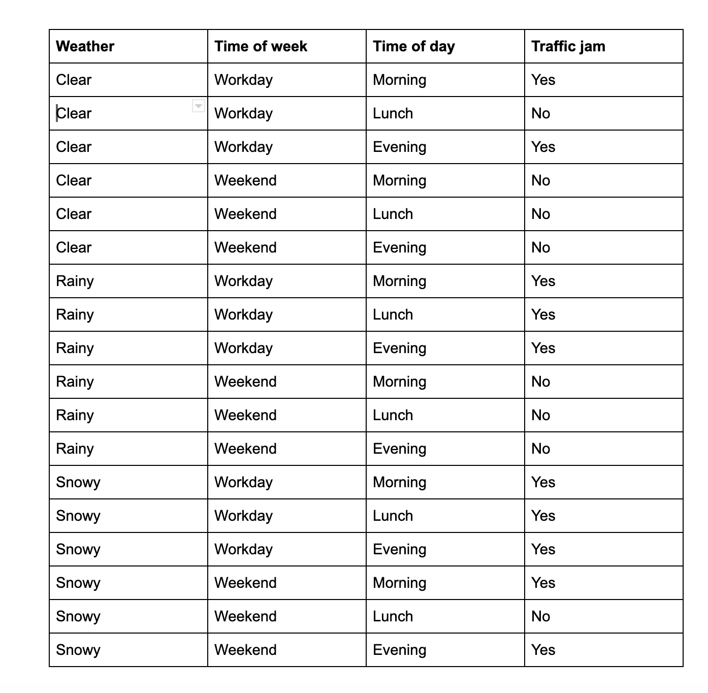
Recently I’ve created a small dummy dataset to use for simple classification tasks. I’ll paste the dataset here again for your convenience.

The purpose of this data is, given 3 facts about a certain moment(the weather, whether it is a weekend or a workday or whether it is morning, lunch or evening), can we predict if there’s a traffic jam in the city?

Decision Tree Classifier in Python with Scikit-Learn

We have 3 dependencies to install for this project, so let’s install them now. Obviously, the first thing we need is the scikit-learn library, and then we need 2 more dependencies which we’ll use for visualization.

pip3 install scikit-learn
pip3 install matplotlib
pip3 install pydotplus

Decision Tree Classifier – installing dependencies

Now let’s import what we need from these packages.

from sklearn import preprocessing
from sklearn import tree
from IPython.display import Image
import pydotplus

Decision Tree Classifier – importing dependencies

def getWeather():
    return ['Clear', 'Clear', 'Clear', 'Clear', 'Clear', 'Clear',
            'Rainy', 'Rainy', 'Rainy', 'Rainy', 'Rainy', 'Rainy',
            'Snowy', 'Snowy', 'Snowy', 'Snowy', 'Snowy', 'Snowy']

def getTimeOfWeek():
    return ['Workday', 'Workday', 'Workday',
            'Weekend', 'Weekend', 'Weekend',
            'Workday', 'Workday', 'Workday',
            'Weekend', 'Weekend', 'Weekend',
            'Workday', 'Workday', 'Workday',
            'Weekend', 'Weekend', 'Weekend']

def getTimeOfDay():
    return ['Morning', 'Lunch', 'Evening',
            'Morning', 'Lunch', 'Evening',
            'Morning', 'Lunch', 'Evening',
            'Morning', 'Lunch', 'Evening',
            'Morning', 'Lunch', 'Evening',
            'Morning', 'Lunch', 'Evening',
            ]

def getTrafficJam():
    return ['Yes', 'No', 'Yes',
            'No', 'No', 'No',
            'Yes', 'Yes', 'Yes',
            'No', 'No', 'No',
            'Yes', 'Yes', 'Yes',
            'Yes', 'No', 'Yes'
            ]

Decision Tree Classifier – loading the data

Decision Tree Classifier – preprocessing

We know that computers have a really hard time when dealing with text and we can make their lives easier by converting the text to numerical values.

Label Encoder

We will use this encoder provided by scikit to transform categorical data from text to numbers. If we have n possible values in our dataset, then LabelEncoder model will transform it into numbers from 0 to n-1 so that each textual value has a number representation.

For example, let’s encode our time of day values.

    timeOfDay = ['Morning', 'Lunch', 'Evening',
            'Morning', 'Lunch', 'Evening',
            'Morning', 'Lunch', 'Evening',
            'Morning', 'Lunch', 'Evening',
            'Morning', 'Lunch', 'Evening',
            'Morning', 'Lunch', 'Evening',
            ]
    labelEncoder = preprocessing.LabelEncoder()
    encodedTimeOfDay = labelEncoder.fit_transform(timeOfDay)
    print (encodedTimeOfDay)
    
    # Prints [2 1 0 2 1 0 2 1 0 2 1 0 2 1 0 2 1 0]

Decision Tree Classifier – encoding our data

Training the Decision Tree Classifier model

Now let’s train our model. So remember, since all our features are textual values, we need to encode all our values and only then we can jump to training.

if __name__=="__main__":
    # Get the data
    weather = getWeather()
    timeOfWeek = getTimeOfWeek()
    timeOfDay = getTimeOfDay()
    trafficJam = getTrafficJam()

    labelEncoder = preprocessing.LabelEncoder()

    # Encode the features and the labels
    encodedWeather = labelEncoder.fit_transform(weather)
    encodedTimeOfWeek = labelEncoder.fit_transform(timeOfWeek)
    encodedTimeOfDay = labelEncoder.fit_transform(timeOfDay)
    encodedTrafficJam = labelEncoder.fit_transform(trafficJam)

    # Build the features
    features = []
    for i in range(len(encodedWeather)):
        features.append([encodedWeather[i], encodedTimeOfWeek[i], encodedTimeOfDay[i]])

    classifier = tree.DecisionTreeClassifier()
    classifier = classifier.fit(features, encodedTrafficJam)

Decision Tree Classifier – training our model

Using our Decision Tree model for predictions

Now we can use the model we have trained to make predictions about the traffic jam.

    # ["Snowy", "Workday", "Morning"]
    print(classifier.predict([[2, 1, 2]]))
    # Prints [1], meaning "Yes"
    # ["Clear", "Weekend", "Lunch"]
    print(classifier.predict([[0, 0, 1]]))
    # Prints [0], meaning "No"

Decision Tree Classifier – making predictions

And it seems to be working! It correctly predicts the traffic jam situations given our data.

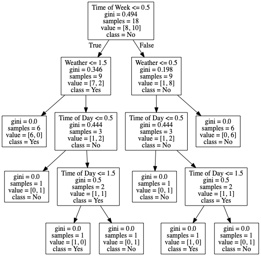
Decision Tree Visualisation

Scikit also provides us with a way of visualizing a Decision Tree model. Here’s a quick helper method I wrote to generate a png image from our decision tree.

def printTree(classifier):
    feature_names = ['Weather', 'Time of Week', 'Time of Day']
    target_names = ['Yes', 'No']
    # Build the daya
    dot_data = tree.export_graphviz(classifier, out_file=None,
                                    feature_names=feature_names,
                                    class_names=target_names)
    # Build the graph
    graph = pydotplus.graph_from_dot_data(dot_data)

    # Show the image
    Image(graph.create_png())
    graph.write_png("tree.png")

Decision Tree Classifier – visualizing the decision tree

And here’s the result from that.

An easy descriptive statistics approach to summarize the numeric and categoric data variables through the Measures of Central Tendency and Measures of Spread for every Exploratory Data Analysis process.

About the Exploratory Data Analysis (EDA)

EDA is the first step in the data analysis process. It allows us to understand the data we are dealing with by describing and summarizing the dataset’s main characteristics, often through visual methods like bar and pie charts, histograms, boxplots, scatterplots, heatmaps, and many more.

Why is EDA important?

• Maximize insight into a dataset (be able to listen to your data)
• Uncover underlying structure/patterns
• Detect outliers and anomalies
• Extract and select important variables
• Increase computational effenciency
• Test underlying assumptions (e.g. business intuiton)

Moreover, to be capable of exploring and explain the dataset’s features with all its attributes getting insights and efficient numeric summaries of the data, we need help from Descriptive Statistics.

Statistics is divided into two major areas:

• Descriptive statistics: describe and summarize data;
• Inferential statistics: methods for using sample data to make general conclusions (inferences) about populations.

This tutorial focuses on descriptive statistics of both numerical and categorical variables and is divided into two parts:

• Measures of central tendency;
• Measures of spread.

Descriptive statistics

Also named Univariate Analysis (one feature analysis at a time), descriptive statistics, in short, help describe and understand the features of a specific dataset, by giving short numeric summaries about the sample and measures of the data.

Descriptive statistics are mere exploration as they do not allows us to make conclusions beyond the data we have analysed or reach conclusions regarding any hypotheses we might have made.

Numerical and categorical variables, as we will see shortly, have different descriptive statistics approaches.

Let’s review the type of variables:

• Numerical continuous: The values are not countable and have an infinite number of possibilities (Someone’s age: 25 years, 4 days, 11 hours, 24 minutes, 5 seconds and so on to the infinite).
• Numerical discrete: The values are countable and have an finite number of possibilities (It is impossible to count 27.52 countries in the EU).
• Categorical ordinal: There is an order implied in the levels (January comes always before February and after December).
• Categorical nominal: There is no order implied in the levels (Female/male, or the wind direction: north, south, east, west).

Numerical variables

• Measures of central tendency: Mean, median
• Measures of spread: Standard deviation, variance, percentiles, maximum, minimum, skewness, kurtosis
• Others: Size, unique, number of uniques

One approach to display the data is through a boxplot. It gives you the 5-basic-stats, such as the minimum, the 1st quartile (25th percentile), the median, the 3rd quartile (75th percentile), and the maximum.

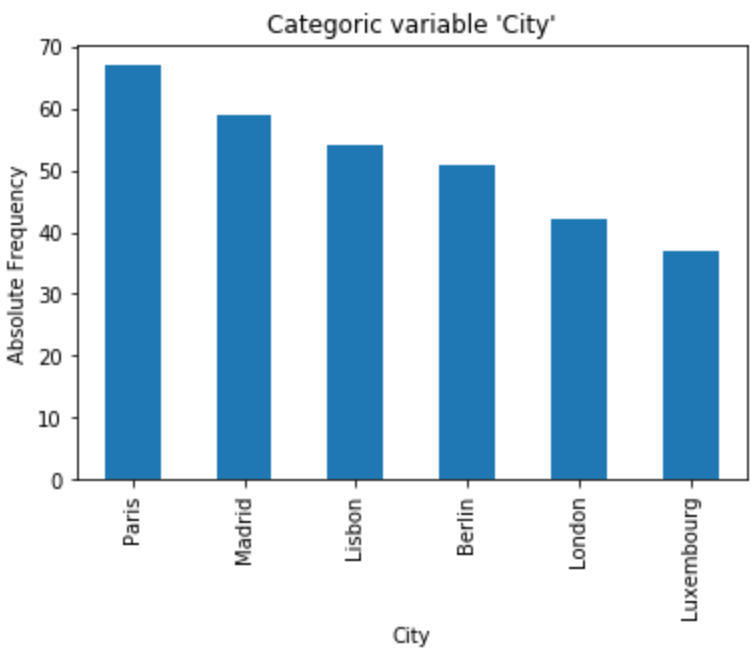
Categorical variables

• Measures of central tendency: Mode (most common)
• Measures of spread: Number of uniques
• Others: Size, % Highest unique

Understanding:

Measures of central tendency

• Mean (average): The total sum of values divided by the total observations. The mean is highly sensitive to the outliers.
• Median (center value): The total count of an ordered sequence of numbers divided by 2. The median is not affected by the outliers.
• Mode (most common): The values most frequently observed. There can be more than one modal value in the same variable.

Measures of spread

• Variance (variability from the mean): The square of the standard deviation. It is also affected by outliers.
• Standard deviation (concentrated around the mean): The standard amount of deviation (distance) from the mean. The std is affected by the outliers. It is the square root of the variance.
• Percentiles: The value below which a percentage of data falls. The 0th percentile is the minimum value, the 100th is the maximum, the 50th is the median.
• Minimum: The smallest or lowest value.
• Maximum: The greatest or highest value.
• The number of uniques (total distinct): The total amount of distinct observations.
• Uniques (distinct): The distinct values or groups of values observed.
• Skewness (symmetric): How much a distribution derives from the normal distribution.
  >> Explained Skew concept in the next section.
• Kurtosis (volume of outliers): How long are the tails and how sharp is the peak of the distribution.
  >> Explained Kurtosis concept in the next section.

Others

• Count (size): The total sum of observations. Counting is also necessary for calculating the mean, median, and mode.
• % highest unique (relativity): The proportion of the highest unique observation regarding all the unique values or group of values.

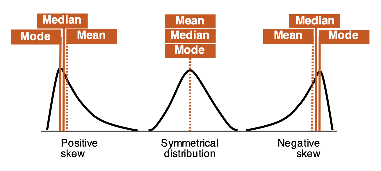
Skewness

In a perfect world, the data’s distribution assumes the form of a bell curve (Gaussian or normally distributed), but in the real world, data distributions usually are not symmetric (= skewed).

Therefore, the skewness indicates how much our distribution derives from the normal distribution (with the skewness value of zero or very close).

There are three generic types of distributions:

• Symmetrical [median = mean]: In a normal distribution, the mean (average) divides the data symmetrically at the median value or close.
• Positive skew [median < mean]: The distribution is asymmetrical, the tail is skewed/longer towards the right-hand side of the curve. In this type, the majority of the observations are concentrated on the left tail, and the value of skewness is positive.
• Negative skew [median > mean]: The distribution is asymmetrical and the tail is skewed/longer towards the left-hand side of the curve. In this type of distribution, the majority of the observations are concentrated on the right tail, and the value of skewness is negative.

Rule of thumbs:

• Symmetric distribution: values between –0.5 to 0.5.
• Moderate skew: values between –1 and -0.5 and 0.5 and 1.
• High skew: values <-1 or >1.

Kurtosis

kurtosis is another useful tool when it comes to quantify the shape of a distribution. It measures both how long are the tails, but most important, and how sharp is the peak of the distributions.

If the distribution has a sharper and taller peak and shorter tails, then it has a higher kurtosis while a low kurtosis can be observed when the peak of the distribution is flatter with thinner tails. There are three types of kurtosis:

• Leptokurtic: The distribution is tall and thin. The value of a leptokurtic must be > 3.
• Mesokurtic: This distribution looks the same or very similar to a normal distribution. The value of a “normal” mesokurtic is = 3.
• Platykurtic: The distributions have a flatter and wider peak and thinner tails, meaning that the data is moderately spread out. The value of a platykurtic must be < 3.

The kurtosis values determine the volume of the outliers only.

Kurtosis is calculated by raising the average of the standardized data to the fourth power. If we raise any standardized number (less than 1) to the 4th power, the result would be a very small number, somewhere close to zero. Such a small value would not contribute much to the kurtosis. The conclusion is that the values that would make a difference to the kurtosis would be the ones far away from the region of the peak, put it in other words, the outliers.

The Jupyter notebook — IPython

In this section, we will be giving short numeric stats summaries concerning the different measures of central tendency and dispersion of the dataset.

let’s work on some practical examples through a descriptive statistics environment in Pandas.

Start by importing the required libraries:

import pandas as pd
import numpy as np
import scipy
import seaborn as sns
import matplotlib.pyplot as plt
%matplotlib inline

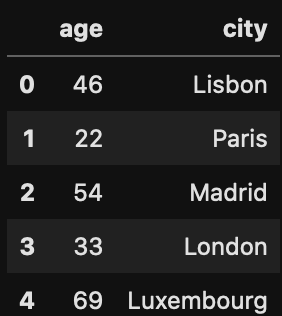
Load the dataset:
df = pd.read_csv("sample.csv", sep=";")

Print the data:
df.head()

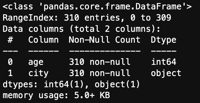
Before any stats calculus, let’s just take a quick look at the data:
df.info

The dataset consists of 310 observations and 2 columns. One of the attributes is numerical, and the other categorical. Both columns have no missing values.

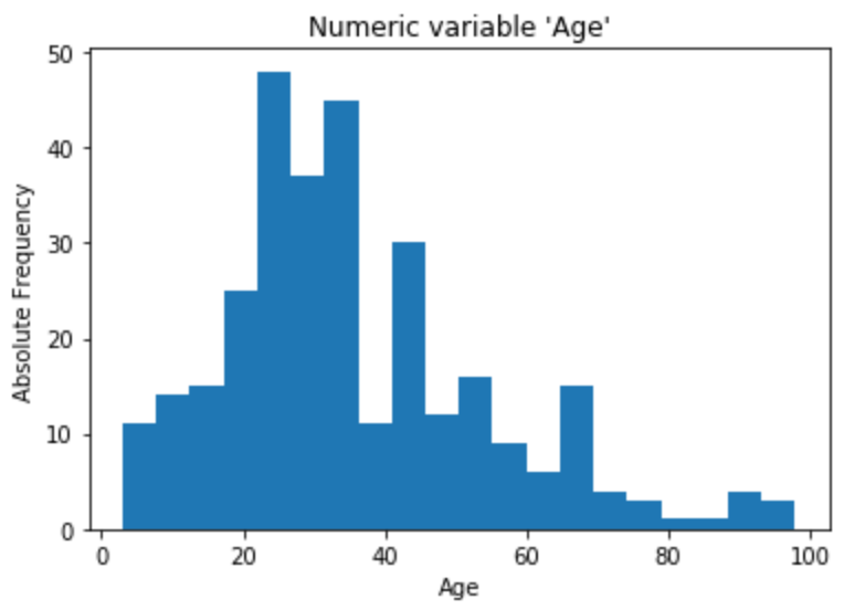
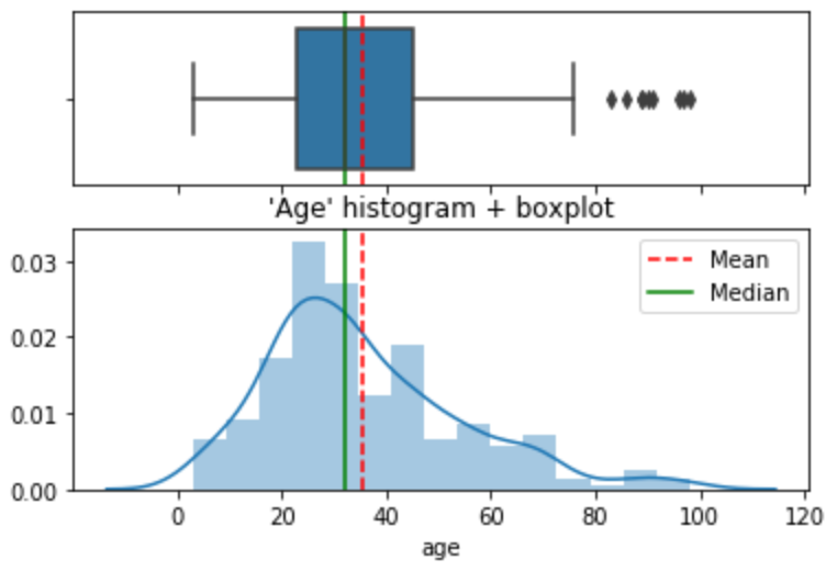
Numerical variable

The numerical variable we are going to analyze is age. First step is to visually observe the variable. So let’s plot an histogram and a boxplot.

plt.hist(df.age, bins=20)
plt.xlabel(“Age”)
plt.ylabel(“Absolute Frequency”)
plt.show()

sns.boxplot(x=age, data=df, orient="h").set(xlabel="Age", title="Numeric variable 'Age'");

It is also possible to visually observe the variable with both a histogram and a boxplot combined. I find it a useful graphical combination and use it a lot in my reports.

age = df.agef, (ax_box, ax_hist) = plt.subplots(2, sharex=True, gridspec_kw= {"height_ratios": (0.8, 1.2)})mean=np.array(age).mean()
median=np.median(age)sns.boxplot(age, ax=ax_box)
ax_box.axvline(mean, color='r', linestyle='--')
ax_box.axvline(median, color='g', linestyle='-')sns.distplot(age, ax=ax_hist)
ax_hist.axvline(mean, color='r', linestyle='--')
ax_hist.axvline(median, color='g', linestyle='-')plt.legend({'Mean':mean,'Median':median})
plt.title("'Age' histogram + boxplot")ax_box.set(xlabel='')
plt.show()

Measures of central tendency

1. Mean:
df.age.mean()

35.564516129032256

2. Median:
df.age.median()

32.0

Measures of spread

3. Standard deviation:
df.age.std()

18.824363618000913

4. Variance:
df.age.var()

354.3566656227164

5. a) Percentiles 25%:
df.age.quantile(0.25)

23.0

b) Percentile 75%:
df.age.quantile(0.75)

45.0

c) In one go:
df.age.quantile(q=[.25, .75)

0.25    23.0
0.75    45.0
Name: age, dtype: float64

6. Minimum and maximum:
df.age.min(), df.age.max()

(3, 98)

7. Skewness (with scipy):
scipy.stats.skew(df.age)

0.9085582496839909

8. Kurtosis (with scipy):
scipy.stats.kurtosis(df.age)

0.7254158742250474

Others

9. Size (number of rows):
df.age.count()

310

10. Number of uniques (total distinct)
df.age.nunique()

74

11. Uniques (distinct):
df.age.unique()

array([46, 22, 54, 33, 69, 35, 11, 97, 50, 34, 67, 43, 21, 12, 23, 45, 89, 76, 5, 55, 65, 24, 27, 57, 38, 28, 36, 60, 56, 53, 26, 25, 42, 83, 16, 51, 90, 10, 70, 44, 20, 31, 47, 30, 91, 7, 6, 41, 66, 61, 96, 32, 58, 17, 52, 29, 75, 86, 98, 48, 40, 13, 4, 68, 62, 9, 18, 39, 15, 19,  8, 71, 3, 37])

Categorical variable

The categorical variable we are going to analyze is city. Let’s plot a bar chart and get a visual observation of the variable.

df.city.value_counts().plot.bar()
plt.xlabel("City")
plt.ylabel("Absolute Frequency")
plt.title("Categoric variable 'City'")
plt.show()

Measures of central tendency

1. Mode:
df.city.mode()[0]

'Paris'

Measures of spread

2. Number of uniques:
df.city.nunique()

6

3. Uniques (distinct):
df.city.unique()

array(['Lisbon', 'Paris', 'Madrid', 'London', 'Luxembourg', 'Berlin'], dtype=object)

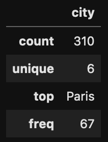
4. Most frequent unique (value count):
df.city.value_counts().head(1)

Paris     67
Name: city, dtype: int64

Others

5. Size (number of rows):
df.city.count()

310

6. % of the highest unique (fraction of the most common unique in regards to all the others):
p = df.city.value_counts(normalize=True)[0]
print(f"{p:.1%}")

21.6%

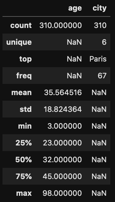
The describe() method shows the descriptive statistics gathered in one table. By default, stats for numeric data. The result is represented as a pandas dataframe.
df.describe()

Adding other non-standard values, for instance, the ‘variance’.
describe_var = data.describe()
describe_var.append(pd.Series(data.var(), name='variance'))

Displaying categorical data.
df.describe(include=["O"])
<=> df.describe(exclude=['float64','int64'])
<=> df.describe(include=[np.object])

By passing the parameter include='all', displays both numeric and categoric variables at once.
df.describe(include='all')

Conclusion

These are the basics of descriptive statistics when developing an exploratory data analysis project with the help of Pandas, Numpy, Scipy, Matplolib and/or Seaborn. When well performed, these stats help us to understand and transform the data for further processing.