Conditional Probability and Unconditional Probability

 

Conditional Probability may be explained as the likelihood of an event or outcome occurring based on the occurrence of a previous event or outcome. Usually, it is calculated by multiplying the probability of the preceding event by the updated probability of the succeeding, or conditional, event.

My general observation says that in problems where the occurrence of one event affects the happening of the following event. These scenarios of probability are classic conditional probability examples.

In the context of mathematics, the probability of occurrence of any event A when another event B in relation to A has already occurred is known as conditional probability.

Our discussion would also include differences between Conditional and Unconditional Probability and round off with the basic differences between Conditional and Joint Probability.

Conditional Probability

Definition of Conditional Probability

The conditional probability may be defined as the probability of one event occurring with some relationship to one or more other events.

It is to be noted that the conditional probability does not state that there is always a causal relationship between the two events, as well as it does not indicate that both events occur simultaneously.

It’s primarily related to the Bayes’ theorem, which is one of the most influential theories in statistics.

The Formula for Conditional Probability may be explained as:

P(A|B) –  the probability of event A occurring given that event B has already occurred

P (A ∩ B) – the joint probability of events A and B; the probability that both events A and B occur at the same time

P(B) – the probability of event B

Formula of Conditional Probability

The formula above is applied to the calculation of the conditional probability of events that are neither independent nor mutually exclusive.

Experts on Conditional Probability suggest another way of calculating it by using the Bayes’ theorem. The theorem can be used to determine the conditional probability of event A, given that the event B has occurred by knowing the conditional probability of event B, given the event A has occurred, as well as the individual probabilities of the event A and B. Mathematically, the Bayes’ theorem can be denoted in the following way:

Baye’s Theorem

Conditional Probability for Independent Events

Conditional Probability may be explained as two events that are independent of each other if the probability of the outcome of one event does not influence the probability of the outcome of another event. Therefore, the two independent events A and B may be represented as:

P(A|B) = P(A)

P(B|A) = P(B)

Conditional Probability of two independent events.

Conditional Probability for Mutually Exclusive Events

In probability theory, mutually exclusive events may be explained as the events that cannot occur simultaneously. In other words, if an event has already occurred, another event cannot occur. Thus, the conditional probability of the mutually exclusive events is always zero.

P(A|B) = 0

P(B|A) = 0

Conditional Probability Examples

Examples using a table of data

According to a research paper, a two-way table of data is one of the most common problems we see in Conditional Probability. Here, we take a look at how to find different probabilities using such a table.

Example

A survey asked full time and part-time students how often they had visited the college’s tutoring center in the last month. The results are shown below.

In a survey conducted by a college both full time and part-time, students were asked how often they had visited the college’s tutoring center in the last two months. The results may be represented as follows:

Conditional Probability Example using Table Data

Suppose that a surveyed student is randomly selected.

(a) What is the probability the student visited the tutoring center four or more times, given that the student is full time?

Conditional probability is all about focusing on the information you know. When calculating this probability, we are given that the student is full time. Therefore, we should only look at full-time students to find the probability.

The probability the student visited the tutoring center four or more times,

(b) Suppose that a student is part-time. What is the probability that the student visited the tutoring center one or fewer times?

This one is a bit trickier, because of the wording. Let us put it in the following way:

Find: probability student visited the tutoring center one or fewer times

Assume or given: a student is part-time (“suppose that a student is part-time”)

The probability that the student visited the tutoring center one or fewer times. The student is part-time.

Since we are assuming (or supposing) the student is part-time, we will only look at part-time students for this calculation.

(c) If the student visited the tutoring center four or more times, what is the probability he or she is a part-time student?

As stated above, we must make sure we know what is given, and what we are finding.

Find probability he or she is part-time

Assume or given: the student visited the tutoring center four or more times (“if the student visited the tutoring center four or more times…”)

For this question, we are only looking at students who visited the tutoring center four or more times.

The probability that the student is a part-time assuming that the student visited the tutoring center four or more times

Difference between Conditional & Joint Probability

What is Joint Probability

The joint probability may be explained as a measure of how likely it is for two (or more) things to occur.  For instance, if you roll two dice, you have the probability of getting a six on the first and a four on the second. This is a classic example of   Joint Probability, where the probability of occurrence of both results is possible.

What is Conditional Probability

Conditional probability, on the other hand, maybe explained as a measure of how likely one situation is likely to happen if you are aware of the occurrence of another event.  

For example, what is the probability that the second die shows a four if the sum of the numbers on the two dice is ten? If you know that the sum is ten, it turns out that it is far more likely that the second die is a four than if you knew nothing about the sum.

Difference between Conditional & Joint Probability

Difference between Conditional & Unconditional Probability

Definition of Conditional Probability

Conditional Probability may be explained as a probability that considers some other piece of information, knowledge, or evidence.

Definition of Unconditional Probability

Unconditional Probability may be explained as a probability that does not consider any other information, knowledge, or evidence.

Krishna Singh, an expert on mathematics and statistics, explains the difference between Conditional and Unconditional Probability with the following example:

Conditional Probability Examples

Pulling an ace out of a deck of cards and then drawing a second ace without replacing the first. You would have a 4/52 chance of getting the first ace, but a 4/51 chance (if you didn’t pull an ace) of the second, making the second conditional upon the results of the first.

Unconditional Probability Examples

Rolling a die. The fact that you got a 6 on one roll has no effect on whether you will roll a 6 later on.

Data Collection, Data Processing & Finished Result

Data Science and Conditional Probability

Data Science often uses statistical inferences to predict or analyze trends from data, while statistical inferences make use of probability distributions of data. Therefore, knowing probability and its applications are important to work effectively on data

Most data science techniques rely on Bayes’ theorem. Bayes’ theorem is a formula that describes at large how to update the probabilities of hypotheses when given evidence. You can build a learner using the Bayes’ theorem to predicts the probability of the response variable belonging to some class, given a new set of attributes.

Data Science is inextricably linked to Conditional Probability. Data Science professionals must have a thorough understanding of probability to solve complicated data science problems. A strong base in Probability and Conditional Probability is essential to fully understand and implement relevant algorithms for use.

Data Science & Conditional Probability

Do you aspire to be a Data Analyst, and then grow further to become a Data Scientist?  Do you like finding answers to complex business challenges interests? Whatever you want, start early to gain a competitive advantage. You must be fluent in the programming languages and tools that will help you get hired.

You may also read my earliest post on How to Create a Killer Data Analyst Resume to create winning CVs that will leave an impression in the mind of the recruiters.

You may start as a Data Analyst, go on to become a Data Scientist with some years of experience, and eventually a data evangelist. Data Science offers lucrative career options. There is enough scope for growth and expansion.

You might be a programmer, a mathematics graduate, or simply a bachelor of Computer Applications. Students with a master’s degree in Economics or Social Science can also be a data scientist. Take up a Data Science or Data Analytics course, to learn Data Science skills and prepare yourself for the Data Scientist job, you have been dreaming of.

A Career in Data Science

Taking up a good Data Science or Data Analytics course teaches you the key Data Science skills and prepares you for the Data Scientist, Data Scientist role (that you aspire for) in the near future. Do not forget to include all your skills in your data scientist’s resume.

In addition, students also get lifetime access to online course matter, 24×7 faculty support, expert advice from industry stalwarts, and assured placement support that prepares them better for the vastly expanding Data Science market.

Perceptron is a single layer neural network and a multi-layer perceptron is called Neural Networks.

Perceptron is a linear classifier (binary). Also, it is used in supervised learning. It helps to classify the given input data. But how the heck it works ?

A normal neural network looks like this as we all know

Get this book 👇

Introduction to Machine Learning with Python: A Guide for Data Scientists

It helped me a lot. 🙌 👍

As you can see it has multiple layers.

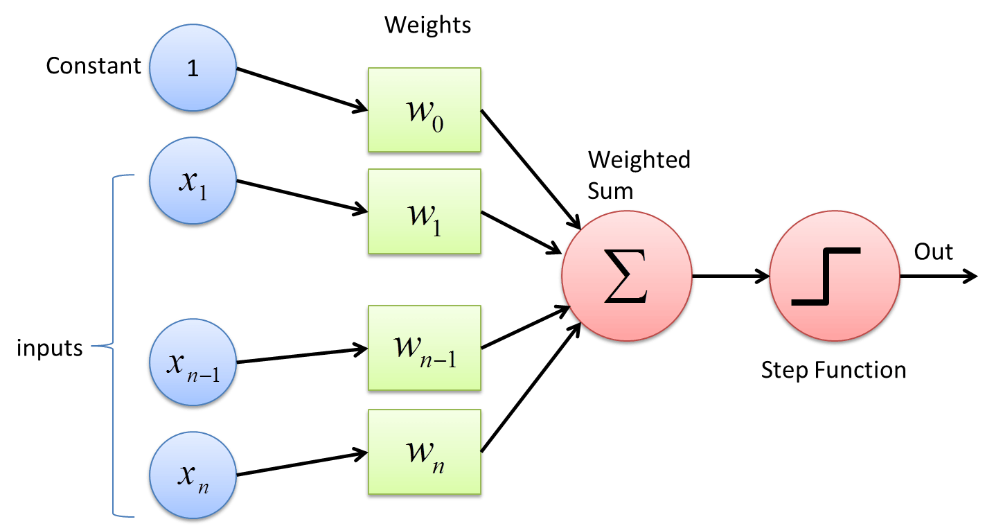
The perceptron consists of 4 parts.

1. Input values or One input layer
2. Weights and Bias
3. Net sum
4. Activation Function

FYI: The Neural Networks work the same way as the perceptron. So, if you want to know how neural network works, learn how perceptron works.

But how does it work?

The perceptron works on these simple steps

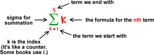
a. All the inputs x are multiplied with their weights w. Let’s call it k.

b. Add all the multiplied values and call them Weighted Sum.

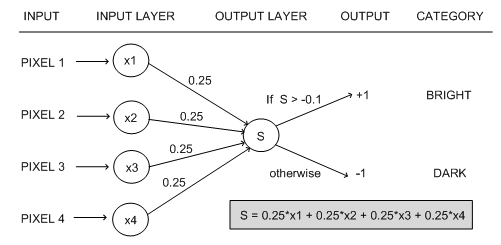
c. Apply that weighted sum to the correct Activation Function.

For Example: Unit Step Activation Function.

---

Why do we need Weights and Bias?

Weights shows the strength of the particular node.

A bias value allows you to shift the activation function curve up or down.

Why do we need Activation Function?

In short, the activation functions are used to map the input between the required values like (0, 1) or (-1, 1).

Where we use Perceptron?

Perceptron is used to classify data into two parts,therefore is known as Linear Binary classifier.

Classification may be defined as the process of predicting class or category from observed values or given data points. The categorized output can have the form such as “Black” or “White” or “spam” or “no spam”.

Mathematically, classification is the task of approximating a mapping function (f) from input variables (X) to output variables (Y). It is basically belongs to the supervised machine learning in which targets are also provided along with the input data set.

An example of classification problem can be the spam detection in emails. There can be only two categories of output, “spam” and “no spam”; hence this is a binary type classification.

To implement this classification, we first need to train the classifier. For this example, “spam” and “no spam” emails would be used as the training data. After successfully train the classifier, it can be used to detect an unknown email.

Types of Learners in Classification

We have two types of learners in respective to classification problems −

Lazy Learners

As the name suggests, such kind of learners waits for the testing data to be appeared after storing the training data. Classification is done only after getting the testing data. They spend less time on training but more time on predicting. Examples of lazy learners are K-nearest neighbor and case-based reasoning.

Eager Learners

As opposite to lazy learners, eager learners construct classification model without waiting for the testing data to be appeared after storing the training data. They spend more time on training but less time on predicting. Examples of eager learners are Decision Trees, Naïve Bayes and Artificial Neural Networks (ANN).

Building a Classifier in Python

Scikit-learn, a Python library for machine learning can be used to build a classifier in Python. The steps for building a classifier in Python are as follows −

Step 1: Importing necessary python package

For building a classifier using scikit-learn, we need to import it. We can import it by using following script −

import sklearn

Step 2: Importing dataset

After importing necessary package, we need a dataset to build classification prediction model. We can import it from sklearn dataset or can use other one as per our requirement. We are going to use sklearn’s Breast Cancer Wisconsin Diagnostic Database. We can import it with the help of following script −

from sklearn.datasets import load_breast_cancer

The following script will load the dataset;

data = load_breast_cancer()

We also need to organize the data and it can be done with the help of following scripts −

label_names = data['target_names']
labels = data['target']
feature_names = data['feature_names']
features = data['data']

The following command will print the name of the labels, ‘malignant’ and ‘benign’ in case of our database.

print(label_names)

The output of the above command is the names of the labels −

['malignant' 'benign']

These labels are mapped to binary values 0 and 1. Malignant cancer is represented by 0 and Benign cancer is represented by 1.

The feature names and feature values of these labels can be seen with the help of following commands −

print(feature_names[0])

The output of the above command is the names of the features for label 0 i.e. Malignant cancer −

mean radius

Similarly, names of the features for label can be produced as follows −

print(feature_names[1])

The output of the above command is the names of the features for label 1 i.e. Benign cancer −

mean texture

We can print the features for these labels with the help of following command −

print(features[0])

This will give the following output −

[1.799e+01 1.038e+01 1.228e+02 1.001e+03 1.184e-01 2.776e-01 3.001e-01
 1.471e-01 2.419e-01 7.871e-02 1.095e+00 9.053e-01 8.589e+00 1.534e+02
 6.399e-03 4.904e-02 5.373e-02 1.587e-02 3.003e-02 6.193e-03 2.538e+01
 1.733e+01 1.846e+02 2.019e+03 1.622e-01 6.656e-01 7.119e-01 2.654e-01
 4.601e-01 1.189e-01]

We can print the features for these labels with the help of following command −

print(features[1])

This will give the following output −

[2.057e+01 1.777e+01 1.329e+02 1.326e+03 8.474e-02 7.864e-02 8.690e-02
7.017e-02  1.812e-01 5.667e-02 5.435e-01 7.339e-01 3.398e+00 7.408e+01
5.225e-03  1.308e-02 1.860e-02 1.340e-02 1.389e-02 3.532e-03 2.499e+01
2.341e+01  1.588e+02 1.956e+03 1.238e-01 1.866e-01 2.416e-01 1.860e-01
2.750e-01  8.902e-02]

Step 3: Organizing data into training & testing sets

As we need to test our model on unseen data, we will divide our dataset into two parts: a training set and a test set. We can use train_test_split() function of sklearn python package to split the data into sets. The following command will import the function −

from sklearn.model_selection import train_test_split

Now, next command will split the data into training & testing data. In this example, we are using taking 40 percent of the data for testing purpose and 60 percent of the data for training purpose −

train, test, train_labels, test_labels = 
   train_test_split(features,labels,test_size = 0.40, random_state = 42)

Step 4: Model evaluation

After dividing the data into training and testing we need to build the model. We will be using Naïve Bayes algorithm for this purpose. The following commands will import the GaussianNB module −

from sklearn.naive_bayes import GaussianNB

Now, initialize the model as follows −

gnb = GaussianNB()

Next, with the help of following command we can train the model −

model = gnb.fit(train, train_labels)

Now, for evaluation purpose we need to make predictions. It can be done by using predict() function as follows −

preds = gnb.predict(test)
print(preds)

This will give the following output −

[1 0 0 1 1 0 0 0 1 1 1 0 1 0 1 0 1 1 1 0 1 1 0 1 1 1 1 1 1 0 1 1 1 1 1 1 0
 1 0 1 1 0 1 1 1 1 1 1 1 1 0 0 1 1 1 1 1 0 0 1 1 0 0 1 1 1 0 0 1 1 0 0 1 0
 1 1 1 1 1 1 0 1 1 0 0 0 0 0 1 1 1 1 1 1 1 1 0 0 1 0 0 1 0 0 1 1 1 0 1 1 0
 1 1 0 0 0 1 1 1 0 0 1 1 0 1 0 0 1 1 0 0 0 1 1 1 0 1 1 0 0 1 0 1 1 0 1 0 0
 1 1 1 1 1 1 1 0 0 1 1 1 1 1 1 1 1 1 1 1 1 0 1 1 1 0 1 1 0 1 1 1 1 1 1 0 0
 0 1 1 0 1 0 1 1 1 1 0 1 1 0 1 1 1 0 1 0 0 1 1 1 1 1 1 1 1 0 1 1 1 1 1 0 1
 0 0 1 1 0 1]

The above series of 0s and 1s in output are the predicted values for the Malignant and Benign tumor classes.

Step 5: Finding accuracy

We can find the accuracy of the model build in previous step by comparing the two arrays namely test_labels and preds. We will be using the accuracy_score() function to determine the accuracy.

from sklearn.metrics import accuracy_score
print(accuracy_score(test_labels,preds))
0.951754385965

The above output shows that NaïveBayes classifier is 95.17% accurate.

Classification Evaluation Metrics

The job is not done even if you have finished implementation of your Machine Learning application or model. We must have to find out how effective our model is? There can be different evaluation metrics, but we must choose it carefully because the choice of metrics influences how the performance of a machine learning algorithm is measured and compared.

The following are some of the important classification evaluation metrics among which you can choose based upon your dataset and kind of problem −

Confusion Matrix

• Confusion Matrix − It is the easiest way to measure the performance of a classification problem where the output can be of two or more type of classes.

Various ML Classification Algorithms

The followings are some important ML classification algorithms −

• Logistic Regression
• Support Vector Machine (SVM)
• Decision Tree
• Naïve Bayes
• Random Forest

We will be discussing all these classification algorithms in detail in further chapters.

Applications

Some of the most important applications of classification algorithms are as follows −

• Speech Recognition
• Handwriting Recognition
• Biometric Identification
• Document Classification

Much of modern technology is based on computational models known as artificial neural networks. There are many different types of neural networks which function on the same principles as the nervous system in the human body.

As Howard Rheingold said, “The neural network is this kind of technology that is not an algorithm, it is a network that has weights on it, and you can adjust the weights so that it learns. You teach it through trials.”

What are Artificial Neural Networks?

An artificial neural network is a system of hardware or software that is patterned after the working of neurons in the human brain and nervous system. Artificial neural networks are a variety of deep learning technology which comes under the broad domain of Artificial Intelligence.

Deep learning is a branch of Machine Learning which uses different types of neural networks. These algorithms are inspired by the way our brain functions and therefore many experts believe they are our best shot to moving towards real AI (Artificial Intelligence).

Deep learning is becoming especially exciting now as we have more amounts of data and larger neural networks to work with.

Moreover, the performance of neural networks improves as they grow bigger and work with more and more data, unlike other Machine Learning algorithms which can reach a plateau after a point.

How do Neural Networks work?

A neural network has a large number of processors. These processors operate parallelly but are arranged as tiers. The first tier receives the raw input similar to how the optic nerve receives the raw information in human beings.

Each successive tier then receives input from the tier before it and then passes on its output to the tier after it. The last tier processes the final output.

Small nodes make up each tier. The nodes are highly interconnected with the nodes in the tier before and after. Each node in the neural network has its own sphere of knowledge, including rules that it was programmed with and rules it has learnt by itself.  

The key to the efficacy of neural networks is they are extremely adaptive and learn very quickly. Each node weighs the importance of the input it receives from the nodes before it. The inputs that contribute the most towards the right output are given the highest weight.

What are the Different Types of Neural Networks?

Different types of neural networks use different principles in determining their own rules. There are many types of artificial neural networks, each with their unique strengths. You can take a look at this video to see the different types of neural networks and their applications in detail.

Here are some of the most important types of neural networks and their applications.

1. Feedforward Neural Network – Artificial Neuron

This is one of the simplest types of artificial neural networks. In a feedforward neural network, the data passes through the different input nodes till it reaches the output node.

In other words, data moves in only one direction from the first tier onwards until it reaches the output node. This is also known as a front propagated wave which is usually achieved by using a classifying activation function.

Unlike in more complex types of neural networks, there is no backpropagation and data moves in one direction only. A feedforward neural network may have a single layer or it may have hidden layers.

In a feedforward neural network, the sum of the products of the inputs and their weights are calculated. This is then fed to the output. Here is an example of a single layer feedforward neural network.

Feedforward Neural Network – Artificial Neuron

Feedforward neural networks are used in technologies like face recognition and computer vision. This is because the target classes in these applications are hard to classify.

A simple feedforward neural network is equipped to deal with data which contains a lot of noise. Feedforward neural networks are also relatively simple to maintain.

2. Radial Basis Function Neural Network

A radial basis function considers the distance of any point relative to the centre. Such neural networks have two layers. In the inner layer, the features are combined with the radial basis function.

Then the output of these features is taken into account when calculating the same output in the next time-step. Here is a diagram which represents a radial basis function neural network.

Radial Basis Function Neural Network

The radial basis function neural network is applied extensively in power restoration systems. In recent decades, power systems have become bigger and more complex.

This increases the risk of a blackout. This neural network is used in the power restoration systems in order to restore power in the shortest possible time.

3. Multilayer Perceptron

A multilayer perceptron has three or more layers. It is used to classify data that cannot be separated linearly. It is a type of artificial neural network that is fully connected. This is because every single node in a layer is connected to each node in the following layer.

A multilayer perceptron uses a nonlinear activation function (mainly hyperbolic tangent or logistic function). Here’s what a multilayer perceptron looks like.

Multilayer Perceptron

This type of neural network is applied extensively in speech recognition and machine translation technologies.

4. Convolutional Neural Network

A convolutional neural network(CNN) uses a variation of the multilayer perceptrons. A CNN contains one or more than one convolutional layers. These layers can either be completely interconnected or pooled.

Before passing the result to the next layer, the convolutional layer uses a convolutional operation on the input. Due to this convolutional operation, the network can be much deeper but with much fewer parameters.

Due to this ability, convolutional neural networks show very effective results in image and video recognition, natural language processing, and recommender systems.

Convolutional neural networks also show great results in semantic parsing and paraphrase detection. They are also applied in signal processing and image classification.

CNNs are also being used in image analysis and recognition in agriculture where weather features are extracted from satellites like LSAT to predict the growth and yield of a piece of land. Here’s an image of what a Convolutional Neural Network looks like.

Convolutional Neural Network

5. Recurrent Neural Network(RNN) – Long Short Term Memory

A Recurrent Neural Network is a type of artificial neural network in which the output of a particular layer is saved and fed back to the input. This helps predict the outcome of the layer.

The first layer is formed in the same way as it is in the feedforward network. That is, with the product of the sum of the weights and features. However, in subsequent layers, the recurrent neural network process begins.

From each time-step to the next, each node will remember some information that it had in the previous time-step. In other words, each node acts as a memory cell while computing and carrying out operations. The neural network begins with the front propagation as usual but remembers the information it may need to use later.

If the prediction is wrong, the system self-learns and works towards making the right prediction during the backpropagation. This type of neural network is very effective in text-to-speech conversion technology.  Here’s what a recurrent neural network looks like.

Recurrent Neural Network(RNN) – Long Short Term Memory

6. Modular Neural Network

A modular neural network has a number of different networks that function independently and perform sub-tasks. The different networks do not really interact with or signal each other during the computation process. They work independently towards achieving the output.

As a result, a large and complex computational process can be done significantly faster by breaking it down into independent components. The computation speed increases because the networks are not interacting with or even connected to each other.  Here’s a visual representation of a Modular Neural Network.

Modular Neural Network

7. Sequence-To-Sequence Models

A sequence to sequence model consists of two recurrent neural networks. There’s an encoder that processes the input and a decoder that processes the output. The encoder and decoder can either use the same or different parameters. This model is particularly applicable in those cases where the length of the input data is not the same as the length of the output data.  

Sequence-to-sequence models are applied mainly in chatbots, machine translation, and question answering systems.

Summing up

There are many types of artificial neural networks that operate in different ways to achieve different outcomes. The most important part about neural networks is that they are designed in a way that is similar to how neurons in the brain work.

As a result, they are designed to learn more and improve more with more data and more usage. Unlike traditional machine learning algorithms which tend to stagnate after a certain point, neural networks have the ability to truly grow with more data and more usage.

That’s why many experts believe that different types of neural networks will be the fundamental framework on which next-generation Artificial Intelligence will be built. Thus taking a Machine Learning Course will prove to be a added benefit.

Hopefully, by now you must have understood the concept of Neural Networks and its types. Moreover, if you are also inspired by the opportunity of Machine Learning, enroll in our Machine Learning using Python Course.

Data cleaning can be a tedious task.

It’s the start of a new project and you’re excited to apply some machine learning models.

You take a look at the data and quickly realize it’s an absolute mess.

According to IBM Data Analytics you can expect to spend up to 80% of your time cleaning data.

In this post we’ll walk through a number of different data cleaning tasks using Python’s Pandas library.  Specifically, we’ll focus on probably the biggest data cleaning task, missing values.

After reading this post you’ll be able to more quickly clean data.  We all want to spend less time cleaning data, and more time exploring and modeling.Click here to get the FREE Data Cleaning Cheat Sheet

Sources of Missing Values

Before we dive into code, it’s important to understand the sources of missing data.  Here’s some typical reasons why data is missing:

• User forgot to fill in a field.
• Data was lost while transferring manually from a legacy database.
• There was a programming error.
• Users chose not to fill out a field tied to their beliefs about how the results would be used or interpreted.

As you can see, some of these sources are just simple random mistakes.  Other times, there can be a deeper reason why data is missing.

It’s important to understand these different types of missing data from a statistics point of view.  The type of missing data will influence how you deal with filling in the missing values.

Today we’ll learn how to detect missing values, and do some basic imputation.  For a detailed statistical approach for dealing with missing data, check out these awesome slides from data scientist Matt Brems.

Keep in mind, imputing with a median or mean value is usually a bad idea, so be sure to check out Matt’s slides for the correct approach.

Getting Started

Before you start cleaning a data set, it’s a good idea to just get a general feel for the data.  After that, you can put together a plan to clean the data.

I like to start by asking the following questions:

• What are the features?
• What are the expected types (int, float, string, boolean)?
• Is there obvious missing data (values that Pandas can detect)?
• Is there other types of missing data that’s not so obvious (can’t easily detect with Pandas)?

To show you what I mean, let’s start working through the example.The data we’re going to work with is a very small real estate data.

Here’s a quick look at the data:

This is a much smaller dataset than what you’ll typically work with.  Even though it’s a small dataset, it highlights a lot of real-world situations that you will encounter on projects.

A good way to get a quick feel for the data is to take a look at the first few rows.  Here’s how you would do that in Pandas:

# Importing libraries
import pandas as pd
import numpy as np

# Read csv file into a pandas dataframe
df = pd.read_csv("property data.csv")

# Take a look at the first few rows
print df.head()

Out:
   ST_NUM    ST_NAME OWN_OCCUPIED  NUM_BEDROOMS
0   104.0     PUTNAM            Y           3.0
1   197.0  LEXINGTON            N           3.0
2     NaN  LEXINGTON            N           3.0
3   201.0   BERKELEY          NaN           1.0
4   203.0   BERKELEY            Y           3.0

I know that I said we’ll be working with Pandas, but you can see that I also imported Numpy. We’ll use this a little bit later on to rename some missing values, so we might as well import it now.

After importing the libraries we read the csv file into a Pandas dataframe. You can think of the dataframe as a spreadsheet.

With the .head()method, we can easily see the first few rows.

Now I can answer my original question, what are my features?  It’s pretty easy to infer the following features from the column names:

• ST_NUM: Street number
• ST_NAME: Street name
• OWN_OCCUPIED: Is the residence owner occupied
• NUM_BEDROOMS: Number of bedrooms

We can also answer, what are the expected types?

• ST_NUM: float or int… some sort of numeric type
• ST_NAME: string
• OWN_OCCUPIED: string… Y (“Yes”) or N (“No”)
• NUM_BEDROOMS: float or int, a numeric type

To answer the next two questions, we’ll need to start getting more in-depth width Pandas. Let’s start looking at examples of how to detect missing values

Standard Missing Values

So what do I mean by “standard missing values”? These are missing values that Pandas can detect.

Going back to our original data set, let’s take a look at the “Street Number” column.

In the third column there’s an empty cell. In the seventh row there’s an “NA” value.

Clearly these are both missing values. Let’s see how Pandas deals with these.

# Looking at the ST_NUM column
print df['ST_NUM']
print df['ST_NUM'].isnull()

# Looking at the ST_NUM column
Out:
0    104.0
1    197.0
2      NaN
3    201.0
4    203.0
5    207.0
6      NaN
7    213.0
8    215.0

Out:
0    False
1    False
2     True
3    False
4    False
5    False
6     True
7    False
8    False

Taking a look at the column, we can see that Pandas filled in the blank space with “NA”. Using the isnull() method, we can confirm that both the missing value and “NA” were recognized as missing values. Both boolean responses are True.

This is a simple example, but highlights an important point. Pandas will recognize both empty cells and “NA” types as missing values. In the next section, we’ll take a look at some types that Pandas won’t recognize.

Non-Standard Missing Values

Sometimes it might be the case where there’s missing values that have different formats.

Let’s take a look at the “Number of Bedrooms” column to see what I mean.

In this column, there’s four missing values.

• n/a
• NA
• —
• na

From the previous section, we know that Pandas will recognize “NA” as a missing value, but what about the others? Let’s take a look.

# Looking at the NUM_BEDROOMS column
print df['NUM_BEDROOMS']
print df['NUM_BEDROOMS'].isnull()
Copy

Out:
0      3
1      3
2    n/a
3      1
4      3
5    NaN
6      2
7     --
8     na

Out:
0    False
1    False
2    False
3    False
4    False
5     True
6    False
7    False
8    False

Just like before, Pandas recognized the “NA” as a missing value. Unfortunately, the other types weren’t recognized.

If there’s multiple users manually entering data, then this is a common problem. Maybe i like to use “n/a” but you like to use “na”.

An easy way to detect these various formats is to put them in a list. Then when we import the data, Pandas will recognize them right away. Here’s an example of how we would do that.

# Making a list of missing value types
missing_values = ["n/a", "na", "--"]
df = pd.read_csv("property data.csv", na_values = missing_values)

Now let’s take another look at this column and see what happens.

# Looking at the NUM_BEDROOMS column
print df['NUM_BEDROOMS']
print df['NUM_BEDROOMS'].isnull()

Out:
0    3.0
1    3.0
2    NaN
3    1.0
4    3.0
5    NaN
6    2.0
7    NaN
8    NaN

Out:
0    False
1    False
2     True
3    False
4    False
5     True
6    False
7     True
8     True

This time, all of the different formats were recognized as missing values.

You might not be able to catch all of these right away. As you work through the data and see other types of missing values, you can add them to the list.

It’s important to recognize these non-standard types of missing values for purposes of summarizing and transforming missing values. If you try and count the number of missing values before converting these non-standard types, you could end up missing a lot of missing values.

In the next section we’ll take a look at a more complicated, but very common, type of missing value.

Unexpected Missing Values

So far we’ve seen standard missing values, and non-standard missing values. What if we an unexpected type?

For example, if our feature is expected to be a string, but there’s a numeric type, then technically this is also a missing value.

Let’s take a look at the “Owner Occupied” column to see what I’m talking about.

From our previous examples, we know that Pandas will detect the empty cell in row seven as a missing value. Let’s confirm with some code.

# Looking at the OWN_OCCUPIED column
print df['OWN_OCCUPIED']
print df['OWN_OCCUPIED'].isnull()

# Looking at the ST_NUM column
Out:
0      Y
1      N
2      N
3     12
4      Y
5      Y
6    NaN
7      Y
8      Y

Out:
0    False
1    False
2    False
3    False
4    False
5    False
6     True
7    False
8    False

In the fourth row, there’s the number 12. The response for Owner Occupied should clearly be a string (Y or N), so this numeric type should be a missing value.

This example is a little more complicated so we’ll need to think through a strategy for detecting these types of missing values. There’s a number of different approaches, but here’s the way that I’m going to work thorugh this one.

1. Loop through the OWN_OCCUPIED column
2. Try and turn the entry into an integer
3. If the entry can be changed into an integer, enter a missing value
4. If the number can’t be an integer, we know it’s a string, so keep going

Let’s take a look at the code and then we’ll go through it in detail.

# Detecting numbers 
cnt=0
for row in df['OWN_OCCUPIED']:
    try:
        int(row)
        df.loc[cnt, 'OWN_OCCUPIED']=np.nan
    except ValueError:
        pass
    cnt+=1

In the code we’re looping through each entry in the “Owner Occupied” column. To try and change the entry to an integer, we’re using int(row).

If the value can be changed to an integer, we change the entry to a missing value using Numpy’s np.nan.

On the other hand, if it can’t be changed to an integer, we pass and keep going.

You’ll notice that I used try and except ValueError. This is called exception handling, and we use this to handle errors.

If we were to try and change an entry into an integer and it couldn’t be changed, then a ValueError would be returned, and the code would stop. To deal with this, we use exception handling to recognize these errors, and keep going.

Another important bit of the code is the .loc method. This is the preferred Pandas method for modfiying entries in place. For more info on this you can check out the Pandas documentation.

Now that we’ve worked through the different ways of detecting missing values, we’ll take a look at summarizing, and replacing them.

Summarizing Missing Values

After we’ve cleaned the missing values, we will probably want to summarize them. For instance, we might want to look at the total number of missing values for each feature.

# Total missing values for each feature
print df.isnull().sum()

Out:
ST_NUM          2
ST_NAME         0
OWN_OCCUPIED    2
NUM_BEDROOMS    4

Other times we might want to do a quick check to see if we have any missing values at all.

# Any missing values?
print df.isnull().values.any()

Out:
True

We might also want to get a total count of missing values.

# Total number of missing values
print df.isnull().sum().sum()

Out:
8

Now that we’ve summarized the number of missing values, let’s take a look at doing some simple replacements.

Replacing

Often times you’ll have to figure out how you want to handle missing values.

Sometimes you’ll simply want to delete those rows, other times you’ll replace them.

As I mentioned earlier, this shouldn’t be taken lightly. We’ll go over some basic imputations, but for a detailed statistical approach for dealing with missing data, check out these awesome slides from data scientist Matt Brems.

That being said, maybe you just want to fill in missing values with a single value.

# Replace missing values with a number
df['ST_NUM'].fillna(125, inplace=True)

More likely, you might want to do a location based imputation. Here’s how you would do that.

# Location based replacement
df.loc[2,'ST_NUM'] = 125

A very common way to replace missing values is using a median.

# Replace using median 
median = df['NUM_BEDROOMS'].median()
df['NUM_BEDROOMS'].fillna(median, inplace=True)

We’ve gone over a few simple ways to replace missing values, but be sure to check out Matt’s slides for the proper techniques.

Conclusion

Dealing with messy data is inevitable. Data cleaning is just part of the process on a data science project.

In this article we went over some ways to detect, summarize, and replace missing values.

In the not-so-distant past, a data science team would need a few things to effectively use deep learning: This had the effect of bottlenecking deep learning, limiting it to the few projects that met…
— Read on towardsdatascience.com/deep-learning-isnt-hard-anymore-26db0d4749d7

DL not hard anymore

Advanced machine learning models (e.g., Random Forest, deep learning models, etc.) are generally considered not explainable [1][2]. As described in [1][2][3][4], those models largely remain black…
— Read on towardsdatascience.com/explainable-deep-learning-in-breast-cancer-prediction-ae36c638d2a4

Understanding The Concept of Clustering In Unsupervised Learning <a href=”https://twitter.com/Deola04/status/1224079748617396224?ref_src=twsrc%5Etfw”>February 2, 2020</a></blockquote> </script>

A data frame is a table or a two-dimensional array-like structure in which each column contains values of one variable and each row contains one set of values from each column.

Following are the characteristics of a data frame.

• The column names should be non-empty.
• The row names should be unique.
• The data stored in a data frame can be of numeric, factor or character type.
• Each column should contain same number of data items.

Create Data Frame

# Create the data frame.
emp.data <- data.frame(
   emp_id = c (1:5), 
   emp_name = c("Rick","Dan","Michelle","Ryan","Gary"),
   salary = c(623.3,515.2,611.0,729.0,843.25), 
   
   start_date = as.Date(c("2012-01-01", "2013-09-23", "2014-11-15", "2014-05-11",
      "2015-03-27")),
   stringsAsFactors = FALSE
)
# Print the data frame.			
print(emp.data) 

When we execute the above code, it produces the following result −

 emp_id    emp_name     salary     start_date
1     1     Rick        623.30     2012-01-01
2     2     Dan         515.20     2013-09-23
3     3     Michelle    611.00     2014-11-15
4     4     Ryan        729.00     2014-05-11
5     5     Gary        843.25     2015-03-27

Get the Structure of the Data Frame

The structure of the data frame can be seen by using str() function.

# Create the data frame.
emp.data <- data.frame(
   emp_id = c (1:5), 
   emp_name = c("Rick","Dan","Michelle","Ryan","Gary"),
   salary = c(623.3,515.2,611.0,729.0,843.25), 
   
   start_date = as.Date(c("2012-01-01", "2013-09-23", "2014-11-15", "2014-05-11",
      "2015-03-27")),
   stringsAsFactors = FALSE
)
# Get the structure of the data frame.
str(emp.data)

When we execute the above code, it produces the following result −

'data.frame':   5 obs. of  4 variables:
 $ emp_id    : int  1 2 3 4 5
 $ emp_name  : chr  "Rick" "Dan" "Michelle" "Ryan" ...
 $ salary    : num  623 515 611 729 843
 $ start_date: Date, format: "2012-01-01" "2013-09-23" "2014-11-15" "2014-05-11" ...

Summary of Data in Data Frame

The statistical summary and nature of the data can be obtained by applying summary() function.

# Create the data frame.
emp.data <- data.frame(
   emp_id = c (1:5), 
   emp_name = c("Rick","Dan","Michelle","Ryan","Gary"),
   salary = c(623.3,515.2,611.0,729.0,843.25), 
   
   start_date = as.Date(c("2012-01-01", "2013-09-23", "2014-11-15", "2014-05-11",
      "2015-03-27")),
   stringsAsFactors = FALSE
)
# Print the summary.
print(summary(emp.data))  

When we execute the above code, it produces the following result −

     emp_id    emp_name             salary        start_date        
 Min.   :1   Length:5           Min.   :515.2   Min.   :2012-01-01  
 1st Qu.:2   Class :character   1st Qu.:611.0   1st Qu.:2013-09-23  
 Median :3   Mode  :character   Median :623.3   Median :2014-05-11  
 Mean   :3                      Mean   :664.4   Mean   :2014-01-14  
 3rd Qu.:4                      3rd Qu.:729.0   3rd Qu.:2014-11-15  
 Max.   :5                      Max.   :843.2   Max.   :2015-03-27 

Extract Data from Data Frame

Extract specific column from a data frame using column name.

# Create the data frame.
emp.data <- data.frame(
   emp_id = c (1:5),
   emp_name = c("Rick","Dan","Michelle","Ryan","Gary"),
   salary = c(623.3,515.2,611.0,729.0,843.25),
   
   start_date = as.Date(c("2012-01-01","2013-09-23","2014-11-15","2014-05-11",
      "2015-03-27")),
   stringsAsFactors = FALSE
)
# Extract Specific columns.
result <- data.frame(emp.data$emp_name,emp.data$salary)
print(result)

When we execute the above code, it produces the following result −

  emp.data.emp_name emp.data.salary
1              Rick          623.30
2               Dan          515.20
3          Michelle          611.00
4              Ryan          729.00
5              Gary          843.25

Extract the first two rows and then all columns

# Create the data frame.
emp.data <- data.frame(
   emp_id = c (1:5),
   emp_name = c("Rick","Dan","Michelle","Ryan","Gary"),
   salary = c(623.3,515.2,611.0,729.0,843.25),
   
   start_date = as.Date(c("2012-01-01", "2013-09-23", "2014-11-15", "2014-05-11",
      "2015-03-27")),
   stringsAsFactors = FALSE
)
# Extract first two rows.
result <- emp.data[1:2,]
print(result)

When we execute the above code, it produces the following result −

  emp_id    emp_name   salary    start_date
1      1     Rick      623.3     2012-01-01
2      2     Dan       515.2     2013-09-23

Extract 3^rd and 5^th row with 2^nd and 4^th column

# Create the data frame.
emp.data <- data.frame(
   emp_id = c (1:5), 
   emp_name = c("Rick","Dan","Michelle","Ryan","Gary"),
   salary = c(623.3,515.2,611.0,729.0,843.25), 
   
	start_date = as.Date(c("2012-01-01", "2013-09-23", "2014-11-15", "2014-05-11",
      "2015-03-27")),
   stringsAsFactors = FALSE
)

# Extract 3rd and 5th row with 2nd and 4th column.
result <- emp.data[c(3,5),c(2,4)]
print(result)

When we execute the above code, it produces the following result −

  emp_name start_date
3 Michelle 2014-11-15
5     Gary 2015-03-27

Expand Data Frame

A data frame can be expanded by adding columns and rows.

Add Column

Just add the column vector using a new column name.

# Create the data frame.
emp.data <- data.frame(
   emp_id = c (1:5), 
   emp_name = c("Rick","Dan","Michelle","Ryan","Gary"),
   salary = c(623.3,515.2,611.0,729.0,843.25), 
   
   start_date = as.Date(c("2012-01-01", "2013-09-23", "2014-11-15", "2014-05-11",
      "2015-03-27")),
   stringsAsFactors = FALSE
)

# Add the "dept" coulmn.
emp.data$dept <- c("IT","Operations","IT","HR","Finance")
v <- emp.data
print(v)

When we execute the above code, it produces the following result −

  emp_id   emp_name    salary    start_date       dept
1     1    Rick        623.30    2012-01-01       IT
2     2    Dan         515.20    2013-09-23       Operations
3     3    Michelle    611.00    2014-11-15       IT
4     4    Ryan        729.00    2014-05-11       HR
5     5    Gary        843.25    2015-03-27       Finance

Add Row

To add more rows permanently to an existing data frame, we need to bring in the new rows in the same structure as the existing data frame and use the rbind() function.

In the example below we create a data frame with new rows and merge it with the existing data frame to create the final data frame.

# Create the first data frame.
emp.data <- data.frame(
   emp_id = c (1:5), 
   emp_name = c("Rick","Dan","Michelle","Ryan","Gary"),
   salary = c(623.3,515.2,611.0,729.0,843.25), 
   
   start_date = as.Date(c("2012-01-01", "2013-09-23", "2014-11-15", "2014-05-11",
      "2015-03-27")),
   dept = c("IT","Operations","IT","HR","Finance"),
   stringsAsFactors = FALSE
)

# Create the second data frame
emp.newdata <- 	data.frame(
   emp_id = c (6:8), 
   emp_name = c("Rasmi","Pranab","Tusar"),
   salary = c(578.0,722.5,632.8), 
   start_date = as.Date(c("2013-05-21","2013-07-30","2014-06-17")),
   dept = c("IT","Operations","Fianance"),
   stringsAsFactors = FALSE
)

# Bind the two data frames.
emp.finaldata <- rbind(emp.data,emp.newdata)
print(emp.finaldata)

When we execute the above code, it produces the following result −

  emp_id     emp_name    salary     start_date       dept
1      1     Rick        623.30     2012-01-01       IT
2      2     Dan         515.20     2013-09-23       Operations
3      3     Michelle    611.00     2014-11-15       IT
4      4     Ryan        729.00     2014-05-11       HR
5      5     Gary        843.25     2015-03-27       Finance
6      6     Rasmi       578.00     2013-05-21       IT
7      7     Pranab      722.50     2013-07-30       Operations
8      8     Tusar       632.80     2014-06-17       Fianance

 

Deep Learning vs. Machine Learning: A Simple Explanation – By Ajay Kapoor
— Read on hackernoon.com/deep-learning-vs-machine-learning-a-simple-explanation-47405b3eef08

Deep learning and Machine learning…the difference.